Hypersphere Cosmology. (6) P J Carroll 28/2/2021
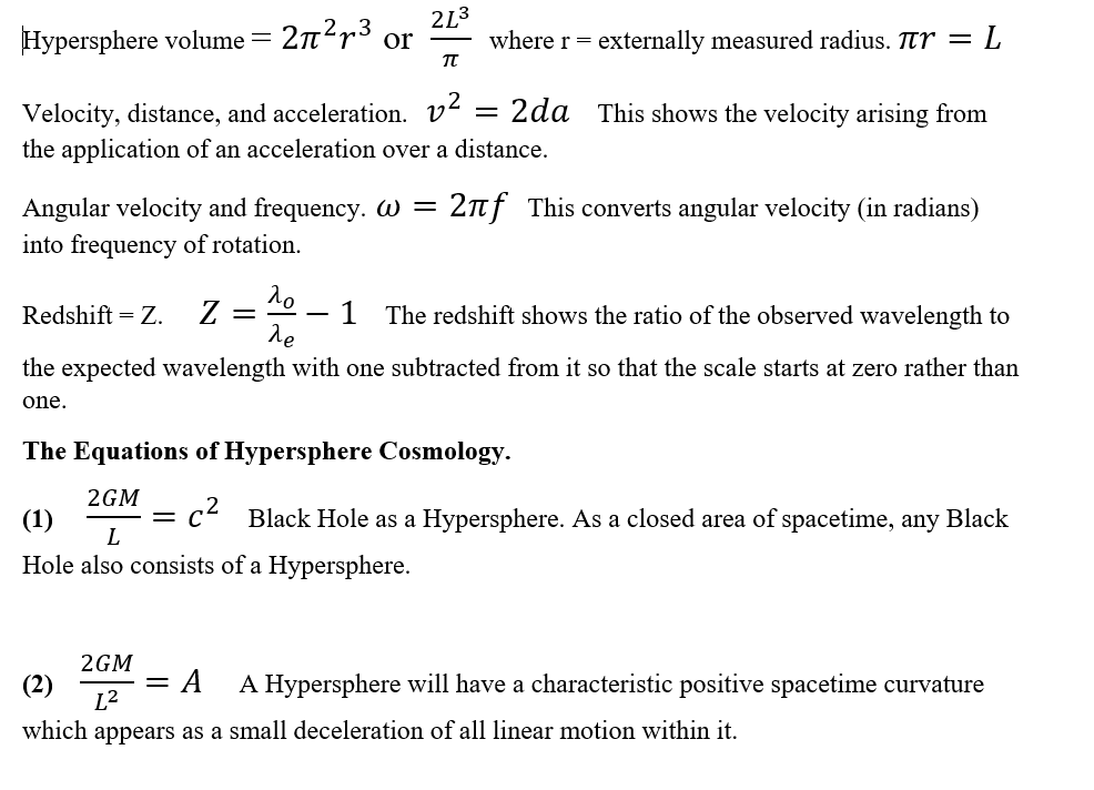
Abstract. Hypersphere Cosmology presents an alternative to the expanding universe of the standard LCDM-Big Bang model. In Hypersphere Cosmology, a universe finite and unbounded in both space and time has a small positive spacetime curvature and a form of rotation. This positive spacetime curvature appears as an acceleration A that accounts for the cosmological redshift of distant galaxies and a stereographic projection of radiant flux from distant sources that makes them appear dimmer and hence more distant.
In Hypersphere Cosmology the universe does not expand, no big bang occurred, singularities do not occur, dark matter and dark energy do not exist. It provides alternative interpretations of the observations that led to such hypotheses.
The seventeen core equations of the theory each have a separate page detailing the physical principles used.
Commentary. The Hypersphere Cosmology model seeks to replace the standard LCDM Big Bang cosmological model with something approaching its exact opposite.
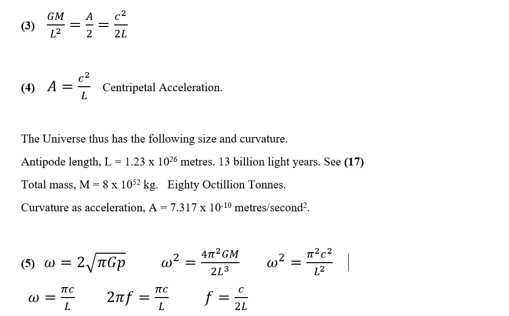
In HC the universe does not expand, it remains as a finite but unbounded structure in both space and time with spatial and temporal horizons of about 13bn light years and 13bn years. The HC universe does not collapse because its major gravitationally bound structures all rotate back and forth to their antipode positions over a 26bnyr period about randomly aligned axes, giving the universe no overall angular momentum and no observable axis of rotation.
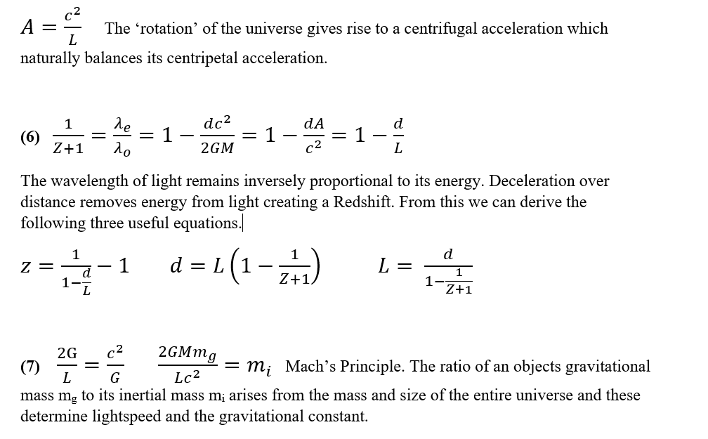
The small positive spacetime curvature of the Glome type Hypersphere of the universe has many effects, it redshifts light traveling across it, it lenses distant objects making them look further away.
In terms of the enormously dimmed flux from very distant sources the antipode will appear to lie an infinite distance away, and beyond direct observation, even though the antipode of any point in the universe lies about 13bnlyr distant.
The antipode thus in a sense plays the anti-role of the Big Bang Singularity in LCDM cosmology. We can never directly observe either, but instead of an apparently infinitely dense and infinitely hot singularity a finite distance away in universe undergoing an accelerating expansion in space and time, Hypersphere Cosmology posits an Antipode that will appear infinitely distant in space and time and infinitely diffuse and cold, even though actual conditions at the antipode of any point will appear broadly similar on the large scale for any observer anywhere in space and time within the hypersphere.
Both HC and LCDM-BB can both model many of the important cosmological observations but in radically different ways. HC has more economical concepts, as a small positive spacetime curvature alone can account for redshift without expansion, the dimming of distant sources of light without an accelerating expansion driven by dark energy, and it also offers a singularity free universe.
Neither model really explains where the universe ‘came from’, but we have no reason to regard non-existence as somehow more fundamental than existence.
The evidence for one-way cosmological evolution remains mixed. The entropy of a vast Glome Hypersphere can remain constant as a function of its hypersurface area. On the very large scale the universe needs only the ability to break neutrons and to break black holes to maintain constant entropy. Very distant parts of the universe appear to contain structures far too large to have evolved in the BB timescale.
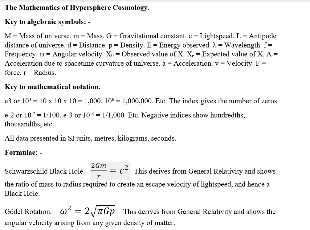
Gödel derived an exact solution of General Relativity in which ‘Matter everywhere rotates relative to the compass of inertia with an angular velocity of twice the square root of pi times the gravitational constant times the density’. This solution became largely ignored because of the apparent lack of observational evidence for an axis of rotation. However, in a hypersphere the galaxies can rotate back and forth to their antipode positions about randomly aligned axes (most probably around the circles of a Hopf Fibration of the hypersphere, thus resulting in a universe with no net overall angular momentum. Such a ‘Vorticitation’ would stabilise a hypersphere against implosion under its own gravity and result in the universe rotating at a mere fraction of an arcsecond per century – well below levels that we can currently observe.
Mach’s Principle can only work in a universe of constant size and density. Strong evidence exists to show that the gravitational constant and inertial masses have remained constant for billions of years.
The Cosmic Microwave Background Radiation may arise from light from this galaxy which re-converges on this galaxy from the antipode in highly redshifted form and smeared out as multiple images around the spherical horizon. Observers in deep intergalactic voids will then not observe such background radiation. Alternatively the Cosmic Microwave Background Radiation may arise from starlight redshifted down to 2.7Kelvin and then kept at that redshift by absorbtion and re-emission by the intergalactic medium at relatively short ranges.
See: -
https://www.specularium.org/component/k2/item/340-the-cmbr
Created by Peter J Carroll. This upgrade 30/11/2021.